The Bias-Variance Tradeoff - Why Being Too Smart is Dumb
So maybe the title is a little clickbaity, I’m sorry, but the concept is important if you ever want to do something useful in machine learning.
Supervised learning
To understand the bias-variance tradeoff, let’s discuss supervised machine learning for one second before moving on.
When doing supervised learning, the idea is to learn to receive input and predict the correct output.

One example of this task is to take an image of a handwritten number and then get the machine to recognize what number it is.

For the computer to learn, you must provide sufficient data examples. One data point is an input and its corresponding output. This is represented below with a gray cube.
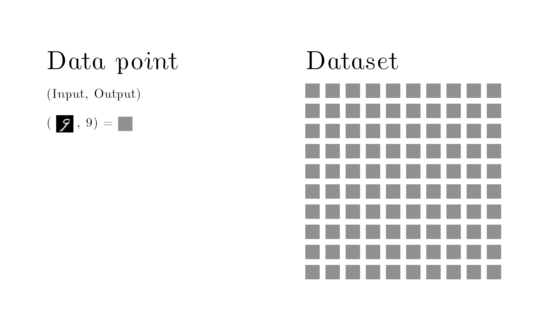
The dataset must contains multiple data points, to achieve a good machine learning model.
You then train the model by continuously feeding the machine these data points and continue tweaking the parameters of the machine learning model to learn from the given examples.
This is kind of like a teacher-to-student scenario where the teacher provides questions and the corresponding correct answer.

After we are done tweaking the model, we take the data points and measure the performance of the model. In other words, we count how often the model correctly classifies an image. It turns out, if you have provided enough data examples and the model is sufficiently complex, the error will go to zero.
An error of zero seems all well and good, right? The error is zero, so we should be done, right? .. Well no .. It’s not good actually because now we have used the same training examples for training and testing. That’s kind of like a student going to an exam with questions the teacher has already answered.
So the machine learning model could have just memorized the answers and not learned anything at all.
Therefore, we must go back and split up the dataset into a training set and a test set.
We only use one set, the training set, for training the algorithm and the other set for testing, the so-called test set. Now we have an appropriate data set for the model - data it has never seen before!
With the test set, we will check how well the model performs once we are done training. So the error on the unseen test set is the golden measurement for checking our machine learning model. And it turns out if we adjust the complexity this time, the error on the test set (green line) will suddenly increase again after dropping. It looks like this:
As seen from the graph, an optimal balance between model complexity and low error on the test set exists in the bottom of the valley. It turns out, model complexity is related to bias and variance. We will see that soon too!
Bias and Variance Decomposition
The error can be decomposed into three things; the bias, the variance, and the noise.

But we can’t get rid of the noise so let’s ignore that. Let’s see why you can decompose the error into bias and variance.
In the following example, a machine learning model is trying to learn to output the number 10. In this example, the number 10 is called the target function y. When a machine learning model tries to estimate y, the estimate is called y hat.

Now comes in a machine learning model, trying to predict the number 10. It turns out, the current model is systematically off target.

Being systematically off target is called bias. Bias is given by:

It’s the true value minus the expectation value and it measures how much we are consistently off.
Now comes in another machine learning model and its predictions are spread everywhere around the target!
Spread is of course a measure of variance. Variance is given by:

This equation doesn’t take into account the actual answer it just measures how spread out the data points are relative to each other.
So that was the two examples where the first model was really biased and the second was highly variant. The error of an actual machine learning model would consist of both bias and variance:
Below is the theoretical error as a function of bias and variance. Adjusting the parameters leads to a minimized error.
With a machine learning model you must try to balance bias and variance as they effect the total error. There exists some mix of bias and variance with an optimal balance. Up until now I haven’t shown you what model complexity is and how it relates to bias and variance let’s do that with yet another example.
Complexity Trade-Off
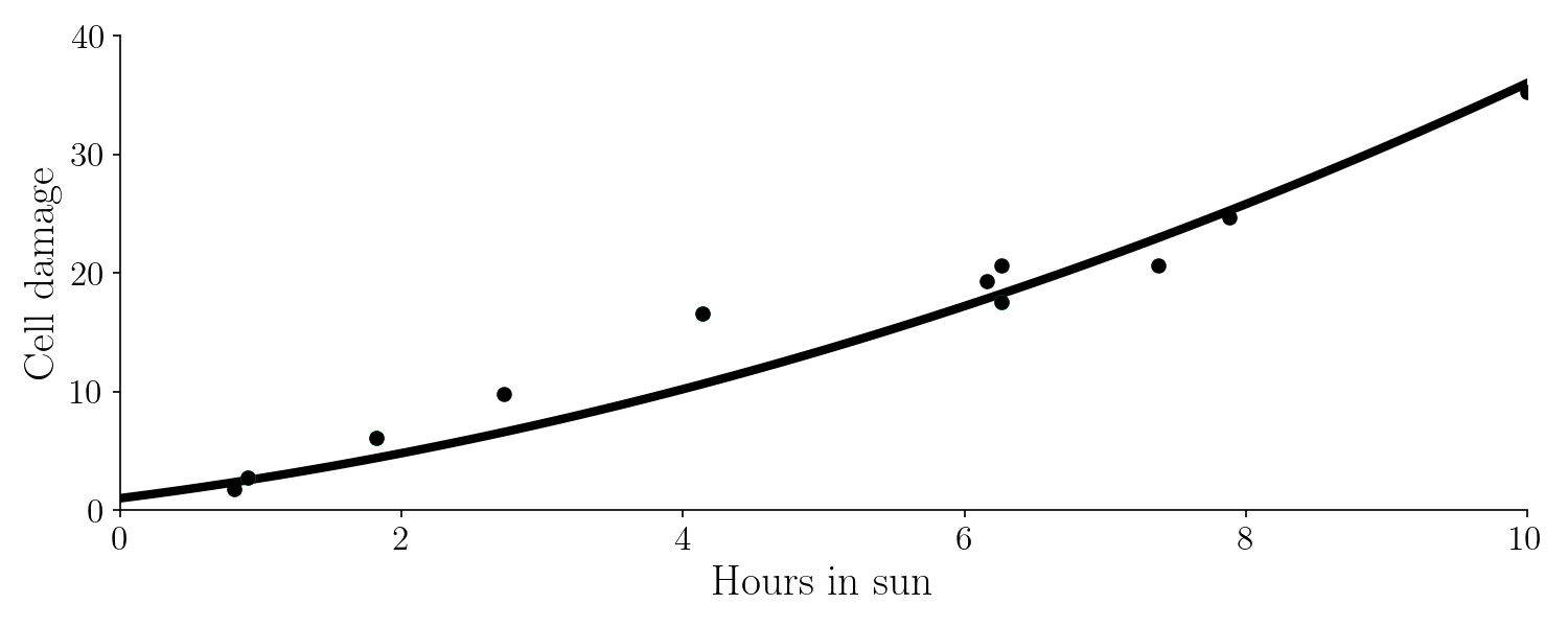
Imagine that we are trying to learn the effect of hours in the sun and the corresponding cell damage in the skin with machine learning. Below is the true function we would like to find (It’s the target function y) :
Of course, knowing the true function is the dream scenario - in reality we will never know this. The target function is a second degree polynomial given by $ f(x) = 0.2 x^2 + 1.5x + 1$, were f(x) is cell damage and x is hours in the sun.
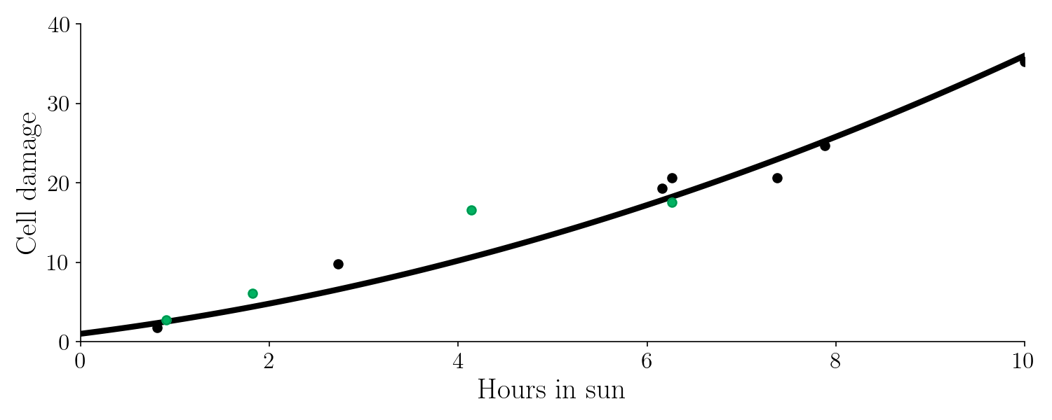
Let’s use machine learning to learn this function. We team up with a doctor that collects the following data points.
The data points can’t be exactly on the true line because of noise and randomness. So this is our data set. As mentioned earlier, we’ll split the data set into a training set (green) and a test set (black).
So now I’ll try to fit the training set with two different polynomials. First, a zero degree polynomial:

So just a number. Second, a 5th degree polynomial:

This is the result:
Let’s have a look on the bias and variance of these different fits, with respect to the test set (green points).
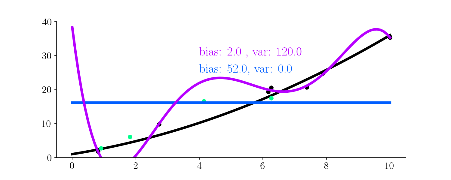
It turns out the 0th degree polynomial is highly highly biased - this machine learning model has underfit as it was not able to capture the patterns in the data. The fifth degree polynomial was highly variant - it began fitting to the noise in the data, making the predictions too variant - the model is overfit.
So somewhere between a 0th degree fit, and a 5th degree fit must be a better function to generalize. Below, I will interpolate from 0th to 5th degree polynomial and fit.
Let’s look at the variance, bias and total error as a function of model complexity (degree of polynomial) for all these fits:
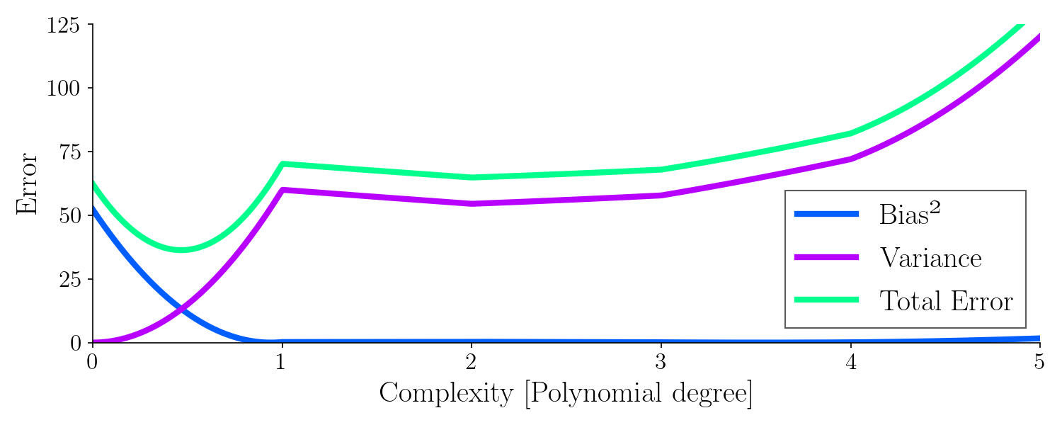
It turns out, the best model to generalize was with a complexity around 0.5, where the total error is minimized. It’s worth noting how the bias drops quickly whereas the variance increases with model complexity.
From this example, hopefully you can see that we must control the bias and the variance in order to make a good machine learning model. This corresponds to adjusting the complexity of the model. Adjusting the complexity influences the tendency of the model to either overfit or underfit.
An overfit model has a low error on the training set but a high error on the test set. An underfit model has a high error on the training set and a high error on the test set as well. So neither is good!
Other Examples
It sounds weird that we’ll need to control or maybe even introduce some bias or variance in order to get a low generalization error.
If the model is not sophisticated enough it doesn’t have high enough complexity / enough learnable parameters, and the model will underfit. On the other side, if the model is too clever / complex it has too many learnable parameters. This will make it too sensitive to the noise in the data set and it will find the wrong patterns, i.e overfit.
Somewhere in between overfit and underfit here is some good balance between being too dumb and too smart.
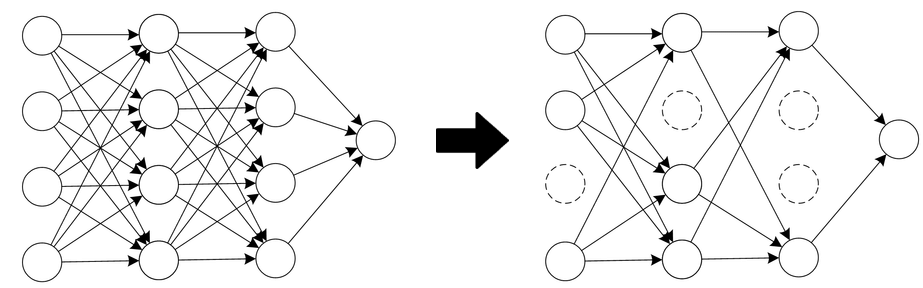
Making a model dumber is called regularization which I showed you by reducing the polynomial degrees in a polynomial fit. An example of regularization in a neural network is dropout, or optimizing via brain damage, where we simply remove connections between neurons to make it dumber:
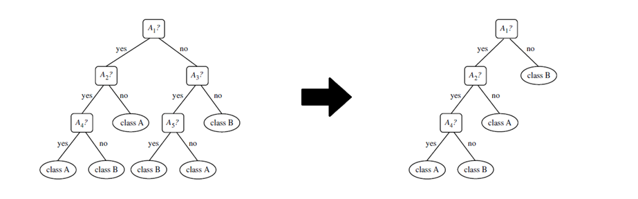
You can also regularize a decision tree by pruning the connections:
There you have it! I showed you via examples why it is a good idea to find a balance between underthinking and overthinking! And now you can make a better machine learning model.
Help me produce more science content by becoming my Patreon or explore the science gifs that are available as a limited NFT supply. Thank you!